Models comparison

In this vignette, we compare the performance of the claim development models implemented in the clmplus package with the performance of the claim amount models available in the apc package (Fannon and Nielsen (2020)). The comparison is performed based on the error incidence on the reserve ( $\text{EI}_R$ , defined below).

The code replicates on a smaller number of datasets the analysis in section 4.3. Benchmarking on Multiple Data Sets of the manuscript Pittarello, Hiabu, and Villegas (2025). We will use publicly available datasets from the R packages clmplus, ChainLadder, and apc for this comparison.

Let us denote with $k,j=0, \ldots, m$ the accident period and the development period respectively. The error incidence on the reserve is defined in the manuscript as the sum of the predicted incremental payments for calendar periods larger than $m$ (the claims reserve, $\sum_{k+j>m} \widehat{X}_{k j}$ ) to the sum of true incremental payments for calendar periods larger than $m$ .

$\text{EI}_R = \left|\frac{\sum_{k+j>m} \widehat{X}_{k j}}{\sum_{k+j>m} X_{k j}}-1\right|.$


list.of.datasets <- list(
  GenIns=GenIns,
  sifa.mod=sifa.mod,
  sifa.gtpl=sifa.gtpl,
  sifa.mtpl=sifa.mtpl,
  amases.gtpl=amases.gtpl,
  amases.mod=amases.mod,
  amases.mtpl=amases.mtpl,
  bz = incr2cum(data.loss.BZ()$response),
  ta = incr2cum(data.loss.TA()$response),
  xl = incr2cum(data.loss.XL()$response),
  vnj = incr2cum(data.loss.VNJ()$response),
  abc=ABC,
  autoC= auto$CommercialAutoPaid,
  autoP = auto$PersonalAutoPaid,
  autoBI = AutoBI$AutoBIPaid,
  mclpaid= MCLpaid,
  medmal=MedMal$MedMalPaid,
  mortgage=Mortgage,
  mw08=MW2008,
  mw14=MW2014, 
  ukmotor = UKMotor,
  usapaid=USAApaid
)

Code for Section 4.3.1. Models Ranking

We rank the different models based on a cross-validation scheme. The training-validation split we use is represented in the following picture.

# models ranking

J=12
df<-data.frame(expand.grid(c(0:(J-1)),c(0:(J-1))),c(1:(J^2)))
colnames(df) <- c("origin","dev","value")
df$value[df$origin+df$dev==(J-1)]=c(2)
df$value[df$origin+df$dev<(J-1)]=c(1)
df$value[df$origin+df$dev>=J]=c(NA)
df[J,3]=c(NA)
df[J*J-J+1,3]=c(NA)

ggplot(data=df, aes(x=as.integer(dev), y=as.integer(origin))) + 
  geom_tile(aes(fill = as.factor(value),color="#000000"))+scale_y_reverse()+
  scale_fill_manual(values=c("royalblue", "darkred", "white"),
                    na.value = "white",
                    labels=c("Train","Validation",""))+
  theme_classic()+
  labs(x="Development year", y="Accident year",fill="")+
  theme(axis.title.x = element_text(size=8), axis.text.x  = element_text(size=7))+
  theme(axis.title.y = element_text(size=8), axis.text.y  = element_text(size=7))+
  scale_color_brewer(guide = 'none')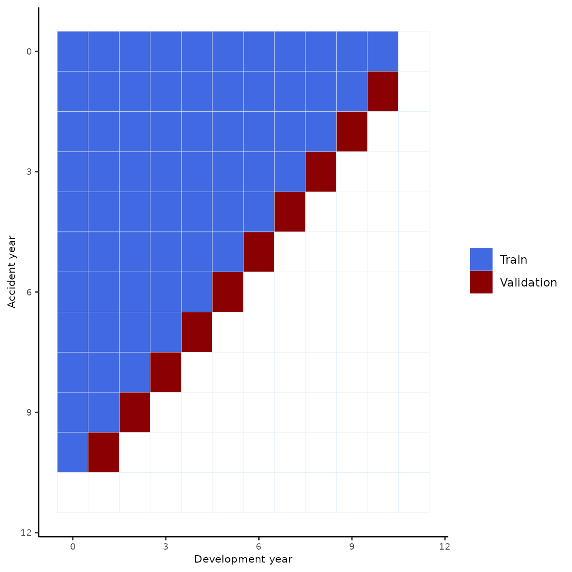

Data split, Train and Validation.


modelsranking.1d <- function(data.T){
  "
  Function to rank the clmplus package and apc package age-period-cohort models.
  
  This function takes a triangle of cumulative payments as input.
  
  It returns the ranking on the triangle.
  "
  
  
  leave.out=1
  
  
  model.name = NULL
  error.incidence = NULL
  mre = NULL
  
  #pre-processing
  triangle <- data.T$cumulative.payments.triangle
  J <- dim(triangle)[2]
  reduced.triangle <- c2t(t2c(triangle)[1:(J-leave.out),1:(J-leave.out)])
  newt.rtt <- AggregateDataPP(reduced.triangle)
  to.project <- t2c(triangle)[1:(J-leave.out-1),J-leave.out]
  true.values <- t2c(triangle)[2:(J-leave.out),J]
  
  
  for(ix in c('a','ac','ap','apc')){
    
    hz.fit <- StMoMo::fit(models[[ix]], 
                          Dxt = newt.rtt$occurrance, 
                          Ext = newt.rtt$exposure,
                          wxt=newt.rtt$fit.w,
                          iterMax=as.integer(1e+05))
    hz.rate = fcst.fn(hz.fit,
                   hazard.model = ix,
                   gk.fc.model = 'a',
                   ckj.fc.model= 'a')$rates[,1]
    
    fij = (2+hz.rate)/(2-hz.rate)
    pred.fij = fij[(leave.out+1):length(fij)]
    pred.v=to.project*pred.fij
    
    r.errors = (pred.v-true.values)/true.values
    error.inc.num = sum(pred.v-true.values,na.rm = T)
    error.inc.den = sum(true.values)
    
    model.name = c(model.name,
                   paste0('clmplus.',ix))
    error.incidence = c(error.incidence,error.inc.num/error.inc.den)
    mre = c(mre,mean(r.errors))
    
    
  }
  
  # ix='lc'
  # hz.fit <- fit.lc.nr(data.T = newt.rtt,
  #                     iter.max = 3e+04)
  # if(hz.fit$converged==TRUE){hz.rate = forecast.lc.nr(hz.fit,J=dim(newt.rtt$cumulative.payments.triangle)[2])$rates[,1:leave.out]
  # fij = (2+hz.rate)/(2-hz.rate)
  # pred.fij = fij[(leave.out+1):length(fij)]
  # pred.v=to.project*pred.fij
  # r.errors = (pred.v-true.values)/true.values
  # 
  # error.inc.num = sum(pred.v-true.values,na.rm = T)
  # error.inc.den = sum(true.values)
  # 
  # model.name = c(model.name,
  #                paste0('clmplus.',ix))
  # error.incidence = c(error.incidence,error.inc.num/error.inc.den)
  # mre = c(mre,mean(r.errors))}
  
  out1 <- data.frame(
    model.name,
    # mre,
    error.incidence)
  
  ## APC package
  
  newt.apc <- apc.data.list(response=newt.rtt$incremental.payments.triangle,
                            data.format="CL")
  
  ## apc
  
  rmse = NULL
  mae = NULL
  error.pc = NULL
  model.name = NULL
  error.incidence = NULL
  model.family = NULL
  mre = NULL
  
  true.inc.values <- t2c(data.T$incremental.payments.triangle)[2:(J-leave.out),(J-leave.out+1):J]
  
  
  for(apc.mods in c("AC","APC")){ #,"AP"
    
    fit <- apc.fit.model(newt.apc,
                         model.family = "od.poisson.response",
                         model.design = apc.mods)
    
    if(apc.mods == "AC"){fcst <- apc.forecast.ac(fit)$trap.response.forecast}
    # if(apc.mods == "AP"){fcst <- apc.forecast.ap(fit)$trap.response.forecast}
    if(apc.mods == "APC"){fcst <- apc.forecast.apc(fit)$trap.response.forecast}
    
    plogram.hat = t2c.full.square(incr2cum(t(fcst)))
    pred.v = plogram.hat[,(J-leave.out+1):J]
    pred.v = pred.v[2:length(pred.v)]
    
    
    r.errors = (pred.v-true.values)/true.values
    error.inc.num = sum(pred.v-true.values)
    error.inc.den = sum(true.values)
    
    model.name = c(model.name,
                   paste0('apc.',tolower(apc.mods)))
    error.incidence = c(error.incidence,error.inc.num/error.inc.den)
    mre = c(mre,mean(r.errors))
    
  }
  
  out2 <- data.frame(
    model.name,
    # mre,
    error.incidence)
  
  out3 <- rbind(out1,out2)
  
  out3 <- out3[order(abs(out3$error.incidence),decreasing = F),]
  out3[,'ei.rank']=c(1:dim(out3)[1])
  # out3[,'mre.rank']=order(abs(out3$mre),decreasing = F)
  #fix it manually
  r2set=min(out3$ei.rank[out3$model.name=='apc.ac'],
            out3$ei.rank[out3$model.name=='clmplus.a'])
  
  out3$ei.rank[out3$model.name=='apc.ac']=r2set
  out3$ei.rank[out3$model.name=='clmplus.a']=r2set
  
  if( out3$ei.rank[out3$model.name=='apc.ac'] < max(out3$ei.rank)){
    cond=out3$ei.rank>out3$ei.rank[out3$model.name=='apc.ac']
    out3$ei.rank[cond]=out3$ei.rank[cond]-1
  }
  
  return(list(models.ranks=out3))
  
}


modelsranking <- function(list.of.datasets){
  
  "
  This functions returns the datasets to plot in the ranking section of the paper.
  
  The input is a list of datasets that constitue the sample. 
  
  The output is the rankings across different data sources.
  "
  
  
  full.ranks=NULL
  
  for(df.ix in names(list.of.datasets)){
    
    out.df=modelsranking.1d(AggregateDataPP(list.of.datasets[[df.ix]]))
    out.df$models.ranks[,'data.source']=rep(df.ix,dim(out.df$models.ranks)[1])
    full.ranks=rbind(full.ranks,out.df$models.ranks)  
  }
  
  return(list(full.ranks=full.ranks))
}

p_min_expd0 <- ggplot(full.ranks$full.ranks, aes(model.name, data.source)) +
   geom_tile(aes(fill = cut(ei.rank, breaks=0:6, labels=1:6)), colour = "grey") +
   ggtitle(" ") +
  theme_classic()+
  geom_text(aes(label = ei.rank))+
   scale_y_discrete(limits=names(list.of.datasets)) +
   scale_fill_manual(drop=FALSE, values=colorRampPalette(c("white","#6699CC"))(6), na.value="#EEEEEE", name="Rank") + 
   xlab("Model") + ylab("Data source")
p_min_expd0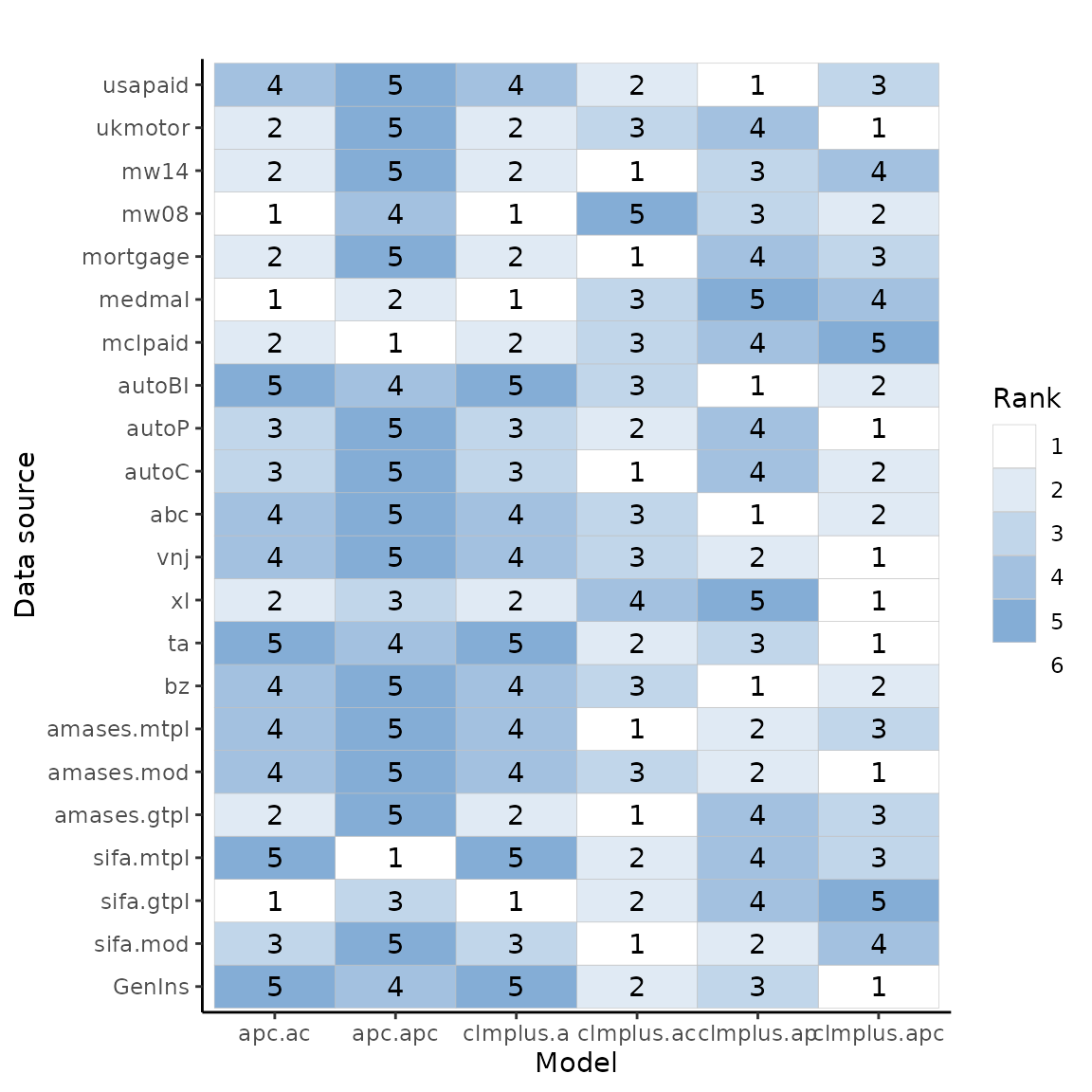

Models ranking plot.

tbl=full.ranks$full.ranks %>%
  dplyr::group_by(model.name) %>%
  dplyr::summarise(mean.rank = mean(ei.rank))
tbl
#> # A tibble: 6 × 2
#>   model.name  mean.rank
#>   <chr>           <dbl>
#> 1 apc.ac           3.09
#> 2 apc.apc          4.14
#> 3 clmplus.a        3.09
#> 4 clmplus.ac       2.32
#> 5 clmplus.ap       3   
#> 6 clmplus.apc      2.45

library(dplyr)
temp.df=full.ranks$full.ranks[,c('model.name','ei.rank')] %>%
  group_by(model.name, ei.rank) %>% summarise(count = n())
#> `summarise()` has grouped output by 'model.name'. You can override using the
#> `.groups` argument.

The following picture was not included in the paper but it shows the models ranks counts for each model.

ggplot(temp.df, aes(y=count, x=factor(ei.rank))) + 
    geom_bar(position="stack", stat="identity",fill='#6699CC') +
  scale_y_continuous(limits=c(0,15))+
  facet_wrap(~model.name, scales='free')+
  theme_classic()+
  ylab("")+
  xlab("Rank")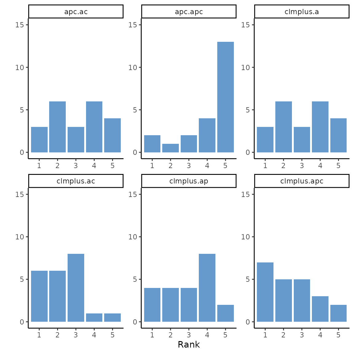

Model rank count.

Code for Section 4.3.2. Model Families Comparison

We evaluate the out-of-sample performance of our models by using a training, validation and testing split.

J=12
df<-data.frame(expand.grid(c(0:(J-1)),c(0:(J-1))),c(1:(J^2)))
colnames(df) <- c("origin","dev","value")
df$value[df$origin+df$dev==(J-1)]=c(3)
df$value[df$origin+df$dev<(J-2)]=c(1)
df$value[df$origin+df$dev==(J-2)]=c(2)
df$value[df$origin+df$dev>=J]=c(NA)
#nas in the lower
df[J,3]=c(NA)
df[J-1,3]=c(NA)
df[J+J-1,3]=c(NA)
df[J*J-J+1,3]=c(NA)
df[J*J-J+1,3]=c(NA)
#nas in the upper tail
df[J*J-J+1-12,3]=c(NA)
df[J*J-J+2-12,3]=c(NA)

ggplot(data=df, aes(x=as.integer(dev), y=as.integer(origin))) + 
  geom_tile(aes(fill = as.factor(value),color="#000000"))+scale_y_reverse()+
  scale_fill_manual(values=c("royalblue", "darkred", "darkgreen","white"),
                    na.value = "white",
                    labels=c("Train","Validation","Test",""))+
  theme_classic()+
  labs(x="Development year", y="Accident year",fill="")+
  theme(axis.title.x = element_text(size=8), axis.text.x  = element_text(size=7))+
  theme(axis.title.y = element_text(size=8), axis.text.y  = element_text(size=7))+
  scale_color_brewer(guide = 'none')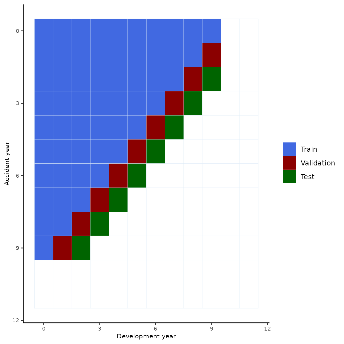

Data split, Train, Validation, and Test.

best.of.the.bests <- function(df1,df2){
  "
  Util to turn character columns values into numeric.
  "
  
  df1=apply(df1,MARGIN=2,FUN=as.numeric)
  df2=apply(df2,MARGIN=2,FUN=as.numeric)
  df3 <- rbind(df1,df2)
  df3=apply(df3,FUN=abs.min,MARGIN = 2)
  
  return(df3)
  
}

modelcomparison.1d <- function(cumulative.payments.triangle){
  "
  Function to compare the clmplus package age-period-cohort models with apc package age-period-cohort models  performances across different triangles.
  
  This function takes a triangle of cumulative payments as input.
  
  It returns the accuracy measures for the two families on the triangle.
  "
  # function internal variables
  
  leave.out=2
  
  rmse = NULL
  mae = NULL
  error.pc = NULL
  model.name = NULL
  error.incidence = NULL
  model.family = NULL
  mre = NULL
  
  # data pre-precessing ----
  
  J <- dim(cumulative.payments.triangle)[2]
  reduced.triangle <- c2t(t2c(cumulative.payments.triangle)[1:(J-leave.out),1:(J-leave.out)])
  newt.rtt <- AggregateDataPP(reduced.triangle)
  
  newt.apc <- apc.data.list(response=newt.rtt$incremental.payments.triangle,
                            data.format="CL")
  
  ## stmomo -----
  to.project <- t2c(cumulative.payments.triangle)[1:(J-leave.out-1),J-leave.out]
  true.values <- t2c(cumulative.payments.triangle)[2:(J-leave.out),(J-leave.out+1):J]
  
  
  for(ix in c('a','ac','ap','apc')){ ##names(models)
    
    hz.fit <- StMoMo::fit(models[[ix]], 
                          Dxt = newt.rtt$occurrance, 
                          Ext = newt.rtt$exposure,
                          wxt=newt.rtt$fit.w,
                          iterMax=as.integer(1e+05))
    hz.rate = fcst.fn(hz.fit,
                   hazard.model = ix,
                   gk.fc.model = 'a',
                   ckj.fc.model= 'a')$rates[,1:leave.out]
    
    J.new=dim(reduced.triangle)[2]
    fij = (2+hz.rate)/(2-hz.rate)
    pred.mx = fij
    pred.mx[,1]=fij[,1]*c(NA,to.project)
    temp=unname(pred.mx[1:(J.new-1),1][!is.na(pred.mx[1:(J.new-1),1])])
    pred.mx[,2]=fij[,2]*c(rep(NA,J.new-length(temp)),temp)
    true.mx= rbind(rep(NA,2),true.values)
    # this is meant to be NA
    true.mx[2,2]=NA
  
    sq.errors = (pred.mx-true.mx)^2
    abs.errors = abs(pred.mx-true.mx)
    r.errors = (pred.mx-true.mx)/true.mx
    error.inc.num = apply(pred.mx-true.mx,sum,MARGIN=2,na.rm=T)
    error.inc.den = apply(true.mx,sum,MARGIN=2,na.rm=T)
    model.name.ix = c(paste0(ix,".val"),paste0(ix,".test"))
    
    model.name = c(model.name,model.name.ix)
    model.family = c(model.family,rep(ix,2))
    rmse = c(rmse,sqrt(apply(sq.errors,MARGIN = 2,mean,na.rm=T)))
    mae = c(mae,apply(abs.errors,MARGIN = 2,mean,na.rm=T))
    mre = c(mre,apply(r.errors,MARGIN = 2,mean,na.rm=T))
    error.incidence = c(error.incidence,error.inc.num/error.inc.den)
    
  }

  
  ## stmomo results ---- 
  
   out1 <- data.frame(
    model.name,
    model.family,
    mre,
    error.incidence,
    rmse,
    mae)
  
  temp.ix <- grepl(".val", model.name)
  temp.df <- out1[temp.ix,]
  
  out2 <- data.frame(
    rmse=temp.df$model.name[which(abs(temp.df$rmse)==min(abs(temp.df$rmse)))],
    mre=temp.df$model.name[which(abs(temp.df$mre)==min(abs(temp.df$mre)))],
    mae=temp.df$model.name[which(abs(temp.df$mae)==min(abs(temp.df$mae)))],
    error.incidence=temp.df$model.name[which(abs(temp.df$error.incidence)==min(abs(temp.df$error.incidence)))])

  
  temp.ix <- grepl(".test", model.name)
  out3 <- out1[temp.ix,]
  
  best.df = out2
  best.df[1,]=NA
  
  out.test.min <- data.frame(
    rmse=out3$model.name[which(abs(out3$rmse)==min(abs(out3$rmse)))],
    mre=out3$model.name[which(abs(out3$mre)==min(abs(out3$mre)))],
    mae=out3$model.name[which(abs(out3$mae)==min(abs(out3$mae)))],
    error.incidence=out3$model.name[which(abs(out3$error.incidence)==min(abs(out3$error.incidence)))])
  
  temp.mx=matrix((sub("\\..*", "", out2) == sub("\\..*", "", out.test.min)),nrow=1)
  choices.mx.clmplus=matrix(sub("\\..*", "", out2),nrow=1)
  
  agreement.frame.clmplus=data.frame(temp.mx)
  choices.frame.clmplus=data.frame(choices.mx.clmplus)
  
  colnames(agreement.frame.clmplus)=colnames(out2)
  colnames(choices.frame.clmplus)=colnames(out2)
  
  for(col.ix in colnames(out2)){
  
  res=out1$model.family[out1$model.name == out2[1,col.ix]]
  res.test = out3$model.family == res
  best.df[1,col.ix] = out3[res.test,col.ix]}
  
  families.set=c('a','apc') #'ap',
  temp.ix = out3$model.family %in% families.set
  comparison.df = out3[temp.ix,]
  comparison.df = cbind(comparison.df,
                        approach=rep('clmplus',length(families.set)))

  
  ## apc ----
  
  rmse = NULL
  mae = NULL
  error.pc = NULL
  model.name = NULL
  error.incidence = NULL
  model.family = NULL
  mre = NULL
  
  true.inc.values <- t2c(cum2incr(cumulative.payments.triangle))[2:(J-leave.out),(J-leave.out+1):J]
  
  
  for(apc.mods in c("AC","APC")){ #,"AP"
    
    fit <- apc.fit.model(newt.apc,
                         model.family = "od.poisson.response",
                         model.design = apc.mods)
    
    if(apc.mods == "AC"){fcst <- apc.forecast.ac(fit)$trap.response.forecast}
    # if(apc.mods == "AP"){fcst <- apc.forecast.ap(fit)$trap.response.forecast}
    if(apc.mods == "APC"){fcst <- apc.forecast.apc(fit)$trap.response.forecast}
    
    plogram.hat = t2c.full.square(incr2cum(t(fcst)))
    pred.mx = plogram.hat[,(J-leave.out+1):J]
    
    # true.mx= rbind(rep(NA,2),true.inc.values)
    # # this is meant to be NA
    # true.mx[2,2]=NA
  
    sq.errors = (pred.mx-true.mx)^2
    abs.errors = abs(pred.mx-true.mx)
    r.errors = (pred.mx-true.mx)/true.mx #use same benchmark
    error.inc.num = apply(pred.mx-true.mx,sum,MARGIN=2,na.rm=T)
    error.inc.den = apply(true.mx,sum,MARGIN=2,na.rm=T) #use same benchmark
    model.name.ix = c(paste0(apc.mods,".val"),paste0(apc.mods,".test"))
    
    model.name = c(model.name,tolower(model.name.ix))
    model.family = c(model.family,tolower(rep(apc.mods,2)))
    rmse = c(rmse,sqrt(apply(sq.errors,MARGIN = 2,mean,na.rm=T)))
    mae = c(mae,apply(abs.errors,MARGIN = 2,mean,na.rm=T))
    mre = c(mre,apply(r.errors,MARGIN = 2,mean,na.rm=T))
    error.incidence = c(error.incidence,error.inc.num/error.inc.den)}
    
      
   out4 <- data.frame(
    model.name,
    model.family,
    mre,
    error.incidence,
    rmse,
    mae)
  
  temp.ix <- grepl(".val", model.name)
  temp.df <- out4[temp.ix,]
  
  out5 <- data.frame(
    rmse=temp.df$model.name[which(abs(temp.df$rmse)==min(abs(temp.df$rmse)))],
    mre=temp.df$model.name[which(abs(temp.df$mre)==min(abs(temp.df$mre)))],
    mae=temp.df$model.name[which(abs(temp.df$mae)==min(abs(temp.df$mae)))],
    error.incidence=temp.df$model.name[which(abs(temp.df$error.incidence)==min(abs(temp.df$error.incidence)))])
  
  temp.ix <- grepl(".test", model.name)
  out6 <- out4[temp.ix,]
  
  out.test.min2 <- data.frame(
  rmse=out6$model.name[which(abs(out6$rmse)==min(abs(out6$rmse)))],
  mre=out6$model.name[which(abs(out6$mre)==min(abs(out6$mre)))],
  mae=out6$model.name[which(abs(out6$mae)==min(abs(out6$mae)))],
  error.incidence=out6$model.name[which(abs(out6$error.incidence)==min(abs(out6$error.incidence)))])

  temp.mx=matrix((sub("\\..*", "", out5) == sub("\\..*", "", out.test.min2)),nrow=1)
  choices.mx.apc=matrix(sub("\\..*", "", out5),nrow=1)
  
  choices.frame.apc=data.frame(choices.mx.apc)
  agreement.frame.apc=data.frame(temp.mx)
  
  colnames(agreement.frame.apc)=colnames(out5)
  colnames(choices.frame.apc)=colnames(out5)
  
  best.df.apc = out5
  best.df.apc[1,]=NA
  
  for(col.ix in colnames(out5)){
  
  res=out4$model.family[out4$model.name == out5[1,col.ix]]
  res.test = out6$model.family == res
  best.df.apc[1,col.ix] = out6[res.test,col.ix]}
      
  families.set=c('ac','apc') #'ap',
  temp.ix = out6$model.family %in% families.set
  comparison.df.apc = out6[temp.ix,]
  comparison.df.apc = cbind(comparison.df.apc,
                            approach=rep('apc',length(families.set)))
  
  
  out = list(
    best.model.clmplus = best.df,
    best.model.apc = best.df.apc,
    agreement.frame.clmplus=agreement.frame.clmplus,
    agreement.frame.apc=agreement.frame.apc,
    choices.frame.clmplus=choices.frame.clmplus,
    choices.frame.apc=choices.frame.apc,
    comparison.df = rbind(comparison.df,
                          comparison.df.apc))
  
  return(out)}


modelcomparison<-function(list.of.datasets){
  "This functions returns the datasets to plot the bake-off section of the paper.
  
  The input is a list of datasets that constitue the sample. 
  
  The output is datasets that contain accuracy measures.
  
  "
  best.fit=NULL
  families.fit=NULL
  agreement.clmplus=NULL
  agreement.apc=NULL
  choices.clmplus=NULL
  choices.apc=NULL
  
  for(df.ix in names(list.of.datasets)){
    cat(paste0(".. Comparison on dataset: ",df.ix))
    out.ix = modelcomparison.1d(list.of.datasets[[df.ix]])
    
    best.of.the.bests.df=best.of.the.bests(out.ix$best.model.clmplus,
                                        out.ix$best.model.apc)
    
    out.ix$best.model.clmplus['package']= 'clmplus'
    out.ix$best.model.apc['package']= 'apc'
    best.of.the.bests.df['package']='overall.best'
    
    best.fit=rbind(best.fit,
                   out.ix$best.model.clmplus,
                   out.ix$best.model.apc,
                   best.of.the.bests.df)
    
    families.fit=rbind(families.fit,
                   out.ix$comparison.df)
    
    agreement.clmplus=rbind(agreement.clmplus,
                         out.ix$agreement.frame.clmplus)
    
    agreement.apc=rbind(agreement.apc,
                         out.ix$agreement.frame.apc)
    
    choices.clmplus=rbind(choices.clmplus,
                         out.ix$choices.frame.clmplus)
    
    choices.apc=rbind(choices.apc,
                         out.ix$choices.frame.apc)
  }
  
  best.fit[,1:4]=apply(best.fit[,1:4],MARGIN = 2,FUN = as.numeric)
  
  families.fit[,c('mre',
                  'error.incidence',
                  'rmse',
                  'mae')]=apply(
                    families.fit[,c('mre',
                                    'error.incidence',
                                    'rmse',
                                    'mae')],
                    MARGIN = 2,
                    FUN = as.numeric)
  
  
  out = list(best.fit=best.fit,
             families.fit=families.fit,
             agreement.clmplus=agreement.clmplus,
             agreement.apc=agreement.apc,
             choices.clmplus=choices.clmplus,
             choices.apc=choices.apc)
  
  return(out)
  
}


bake.off <- function(models.comparison){
  "
  This function plots out the results from the previous computations. 
  
  It takes as input the resulting dataframes of model.comparison.
  
  The output is the boxplots of the paper's bake-off section. 
  
  "
  
  # browser()
  
  p1<- models.comparison$best.fit[,c("rmse","mae","package")] %>%
    tidyr::pivot_longer(-c(package)) %>%
    ggplot(aes(x=package,y=value))+
    geom_boxplot()+
    facet_wrap(.~name,nrow = 1,strip.position = 'bottom')+
    theme_bw()+
    theme(strip.placement = 'outside',strip.background = element_blank())
  
  p2<- models.comparison$best.fit[,c("mre","error.incidence","package")] %>%
    tidyr::pivot_longer(-c(package)) %>%
    ggplot(aes(x=package,y=value))+
    geom_boxplot()+
    facet_wrap(.~name,nrow = 1,strip.position = 'bottom')+
    theme_bw()+
    theme(strip.placement = 'outside',strip.background = element_blank())
  
   abs.best=models.comparison$best.fit[,c("mre","error.incidence","package")]
  abs.best[,c("mre","error.incidence")]=apply(abs.best[,c("mre","error.incidence")],
                                              MARGIN=2,
                                              FUN=abs)
  p3<- abs.best %>%
    tidyr::pivot_longer(-c(package)) %>%
    ggplot(aes(x=package,y=value))+
    geom_boxplot()+
    facet_wrap(.~name,nrow = 1,strip.position = 'bottom')+
    theme_bw()+
    theme(strip.placement = 'outside',strip.background = element_blank())
  
  only.ei=models.comparison$best.fit[,c("error.incidence","package")]
  only.ei[,c("error.incidence")]=abs(only.ei[,c("error.incidence")])
  
  p4<- abs.best %>%
  tidyr::pivot_longer(-c(package)) %>%
  ggplot(aes(x=package,y=value))+
  geom_boxplot()+
  # facet_wrap(.~name,nrow = 1,strip.position = 'bottom')+
  theme_bw()+
  theme(strip.placement = 'outside',strip.background = element_blank())
  
  
  out = list(p1=p1,
             p2=p2,
             p3=p3,
             p4=p4)
  
  return(out)
}

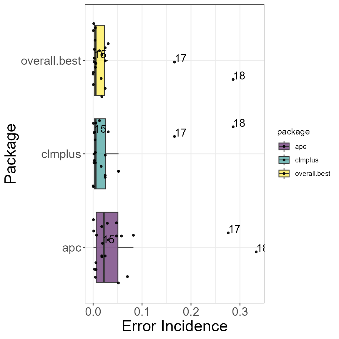
The models in the clmplus package are compared to those in the apc package. Below it can be found the code we used to create the box-plot in figure 8 of our paper.

For each case we are able to pick the best model based on the error incidence.

Error Incidence.

References

Fannon, Zoe, and Bent Nielsen. 2020. Apc: Age-Period-Cohort Analysis. https://CRAN.R-project.org/package=apc.

Pittarello, Gabriele, Munir Hiabu, and Andrés M Villegas. 2025. “Replicating and Extending Chain-Ladder via an Age–Period–Cohort Structure on the Claim Development in a Run-Off Triangle.” North American Actuarial Journal, 1–31.

Gabriele Pittarello

2025-06-12

Code for Section 4.3.1. Models Ranking

Code for Section 4.3.2. Model Families Comparison

References