Vignette 1

Introduction

The clmplus package aims to offer a fast and user-friendly implementation of the modeling framework introduced in our paper, Pittarello, Hiabu, and Villegas (2025).

In this vignette:

We replicate the chain-ladder model using an age-model for the claim development. We can replicate the chain ladder model using an age-model for the claim development. As discussed in the paper, modeling claim development allows us to replicate chain-ladder estimate for claims reserve using fewer parameters than modeling claim amounts (England and Verrall (1999)).
We provide an example illustrating how incorporating a cohort effect can enhance model fit.

Before proceeding, we summarise in a table the notation of the claim development models implemented in clmplus package. The implementation of the models for the claim development available in the clmplus is based on the implementation of the models for human mortality implemented in the StMoMo package. Users can either rely on our default models or set their own configuration for the claim development.

Model	Lexis dimension	Claims reserving
a	age	development (chain-ladder model)
ac	age-cohort	development-accident
ap	age-period	development-calendar
apc	age-period-cohort	development-calendar-accident

Replicate the chain-ladder with the `clmplus` package

For this tutorial, we use the AutoBIPaid run-off triangle available in the ChainLadder package (Gesmann et al. (2025)). Please make sure that the ChainLadder package is installed on your computer before executing the following code.

The data is pre-processed using the AggregateDataPP method.

The desired model is fit using the clmplus method.

a.model.fit=clmplus(AggregateDataPP =  pp_data, 
             hazard.model = "a")
#> StMoMo: The following ages have been zero weighted: 1 
#> StMoMo: The following years have been zero weighted: 1 
#> StMoMo: The following cohorts have been zero weighted: -7 -6 -5 -4 -3 -2 -1 7 
#> StMoMo: Start fitting with gnm
#> StMoMo: Finish fitting with gnm

Out of the fitted model, it is possible to extract the fitted development factors:


a.model.fit$fitted_development_factors
#>      [,1]     [,2]     [,3]     [,4]     [,5]     [,6]     [,7]     [,8]
#> [1,]   NA 4.098156 2.087506 1.619294 1.414518 1.302461 1.236005 1.191122
#> [2,]   NA 4.098156 2.087506 1.619294 1.414518 1.302461 1.236005       NA
#> [3,]   NA 4.098156 2.087506 1.619294 1.414518 1.302461       NA       NA
#> [4,]   NA 4.098156 2.087506 1.619294 1.414518       NA       NA       NA
#> [5,]   NA 4.098156 2.087506 1.619294       NA       NA       NA       NA
#> [6,]   NA 4.098156 2.087506       NA       NA       NA       NA       NA
#> [7,]   NA 4.098156       NA       NA       NA       NA       NA       NA
#> [8,]   NA       NA       NA       NA       NA       NA       NA       NA

It is also possible to extract the fitted effects on the claims development.


a.model.fit$fitted_effects
#> $fitted_development_effect
#>          0          1          2          3          4          5          6 
#>         NA  0.1950754 -0.3503294 -0.7489324 -1.0689916 -1.3366344 -1.5554467 
#>          7 
#> -1.7461089 
#> 
#> $fitted_calendar_effect
#> NULL
#> 
#> $fitted_accident_effect
#> NULL

Predictions can be computed with the predict method.


a.model <- predict(a.model.fit)

Out of the model predictions, we can extract the predicted development factors, the full and lower triangle of predicted cumulative claims.


a.model$development_factors_predicted
#>      [,1]     [,2]     [,3]     [,4]     [,5]     [,6]     [,7]     [,8]
#> [1,]   NA       NA       NA       NA       NA       NA       NA       NA
#> [2,]   NA       NA       NA       NA       NA       NA       NA 1.191122
#> [3,]   NA       NA       NA       NA       NA       NA 1.236005 1.191122
#> [4,]   NA       NA       NA       NA       NA 1.302461 1.236005 1.191122
#> [5,]   NA       NA       NA       NA 1.414518 1.302461 1.236005 1.191122
#> [6,]   NA       NA       NA 1.619294 1.414518 1.302461 1.236005 1.191122
#> [7,]   NA       NA 2.087506 1.619294 1.414518 1.302461 1.236005 1.191122
#> [8,]   NA 4.098156 2.087506 1.619294 1.414518 1.302461 1.236005 1.191122


a.model$lower_triangle
#>      [,1]     [,2]     [,3]     [,4]     [,5]     [,6]     [,7]      [,8]
#> [1,]   NA       NA       NA       NA       NA       NA       NA        NA
#> [2,]   NA       NA       NA       NA       NA       NA       NA  74756.02
#> [3,]   NA       NA       NA       NA       NA       NA 75506.30  89937.23
#> [4,]   NA       NA       NA       NA       NA 67786.58 83784.54  99797.62
#> [5,]   NA       NA       NA       NA 55952.67 72876.17 90075.29 107290.68
#> [6,]   NA       NA       NA 35679.53 50469.34 65734.34 81247.96  96776.25
#> [7,]   NA       NA 24926.91 40364.00 57095.61 74364.80 91915.25 109482.29
#> [8,]   NA 11478.94 23962.35 38802.09 54886.26 71487.21 88358.53 105245.81


a.model$full_triangle
#>      [,1]     [,2]     [,3]     [,4]     [,5]     [,6]     [,7]      [,8]
#> [1,] 1904  7302.00 14798.00 23680.00 33392.00 43463.00 53662.00  63918.00
#> [2,] 2235  8496.00 17187.00 27630.00 38976.00 50730.00 62761.00  74756.02
#> [3,] 2441  9789.00 20451.00 33106.00 46854.00 61089.00 75506.30  89937.23
#> [4,] 2503 10676.00 22486.00 36662.00 52045.00 67786.58 83784.54  99797.62
#> [5,] 2838 11550.00 24278.00 39556.00 55952.67 72876.17 90075.29 107290.68
#> [6,] 2405 10263.00 22034.00 35679.53 50469.34 65734.34 81247.96  96776.25
#> [7,] 2759 11941.00 24926.91 40364.00 57095.61 74364.80 91915.25 109482.29
#> [8,] 2801 11478.94 23962.35 38802.09 54886.26 71487.21 88358.53 105245.81

We can also predict for different forecasting horizons. Below predictions for one calendar period ahead. The forecasting horizon can be specified with the forecasting_horizon argument in the predict method.


a.model.2 <- predict(a.model.fit,
                     forecasting_horizon=1)

We compare our estimates with those obtained with the Mack chain-ladder method (Mack (1993)) as implemented in the ChainLadder package. We predict the same reserve as the literature benchmark.

mck.chl <- MackChainLadder(input_data)
ultimate.chl=mck.chl$FullTriangle[,dim(mck.chl$FullTriangle)[2]]
diagonal=rev(t2c(mck.chl$FullTriangle)[,dim(mck.chl$FullTriangle)[2]])

Estimates are gathered in a data.frame for comparison.

data.frame(ultimate.cost.mack=ultimate.chl,
           ultimate.cost.clmplus=a.model$ultimate_cost,
           reserve.mack=ultimate.chl-diagonal,
           reserve.clmplus=a.model$reserve
           )
#>   ultimate.cost.mack ultimate.cost.clmplus reserve.mack reserve.clmplus
#> 1           63918.00              63918.00         0.00            0.00
#> 2           74756.02              74756.02     11995.02        11995.02
#> 3           89937.23              89937.23     28848.23        28848.23
#> 4           99797.62              99797.62     47752.62        47752.62
#> 5          107290.68             107290.68     67734.68        67734.68
#> 6           96776.25              96776.25     74742.25        74742.25
#> 7          109482.29             109482.29     97541.29        97541.29
#> 8          105245.81             105245.81    102444.81       102444.81

cat('\n Total reserve:',
    sum(a.model$reserve))
#> 
#>  Total reserve: 431058.9

Claims reserving with GLMs compared to hazard models

We fit the stochastic model replicating the chain-ladder with an age-cohort GLM for the claim amounts described in England and Verrall (1999) using the apcpackage Fannon and Nielsen (2020).

library(apc)
#> Warning: package 'apc' was built under R version 4.4.3

ds.apc = apc.data.list(cum2incr(dataset),
                       data.format = "CL")

ac.model.apc = apc.fit.model(ds.apc,
                         model.family = "od.poisson.response",
                         model.design = "AC")

Inspect the model coefficients derived from the output:


ac.model.apc$coefficients.canonical[,'Estimate']
#>        level    age slope cohort slope     DD_age_3     DD_age_4     DD_age_5 
#>   7.41596168   0.74105900   0.16519698  -1.16411707  -0.02909890  -0.17467013 
#>     DD_age_6     DD_age_7     DD_age_8  DD_cohort_3  DD_cohort_4  DD_cohort_5 
#>  -0.17533888   0.17408744  -0.55360421   0.02140672  -0.07364998  -0.03603392 
#>  DD_cohort_6  DD_cohort_7  DD_cohort_8 
#>  -0.15911660   0.20095088  -0.17521544

ac.fcst.apc = apc.forecast.ac(ac.model.apc)

data.frame(reserve.mack=ultimate.chl-diagonal,
           reserve.apc=c(0,ac.fcst.apc$response.forecast.coh[,'forecast']),
           reserve.clmplus=a.model$reserve
           
           )
#>   reserve.mack reserve.apc reserve.clmplus
#> 1         0.00     0.00000            0.00
#> 2     11995.02    67.23865        11995.02
#> 3     28848.23   345.18727        28848.23
#> 4     47752.62   940.68770        47752.62
#> 5     67734.68  2350.85562        67734.68
#> 6     74742.25  4466.77443        74742.25
#> 7     97541.29  9103.24335        97541.29
#> 8    102444.81 14480.43832       102444.81

Our method is able to replicate the chain-ladder results without adding the cohort component.

a.model.fit$fitted_effects
#> $fitted_development_effect
#>          0          1          2          3          4          5          6 
#>         NA  0.1950754 -0.3503294 -0.7489324 -1.0689916 -1.3366344 -1.5554467 
#>          7 
#> -1.7461089 
#> 
#> $fitted_calendar_effect
#> NULL
#> 
#> $fitted_accident_effect
#> NULL

Further inspection can be performed with the clmplus package, which provides the graphical tools to inspect the fitted effects. The fitted effects can be plotted using the plot function on the output of the predict method.

plot(a.model)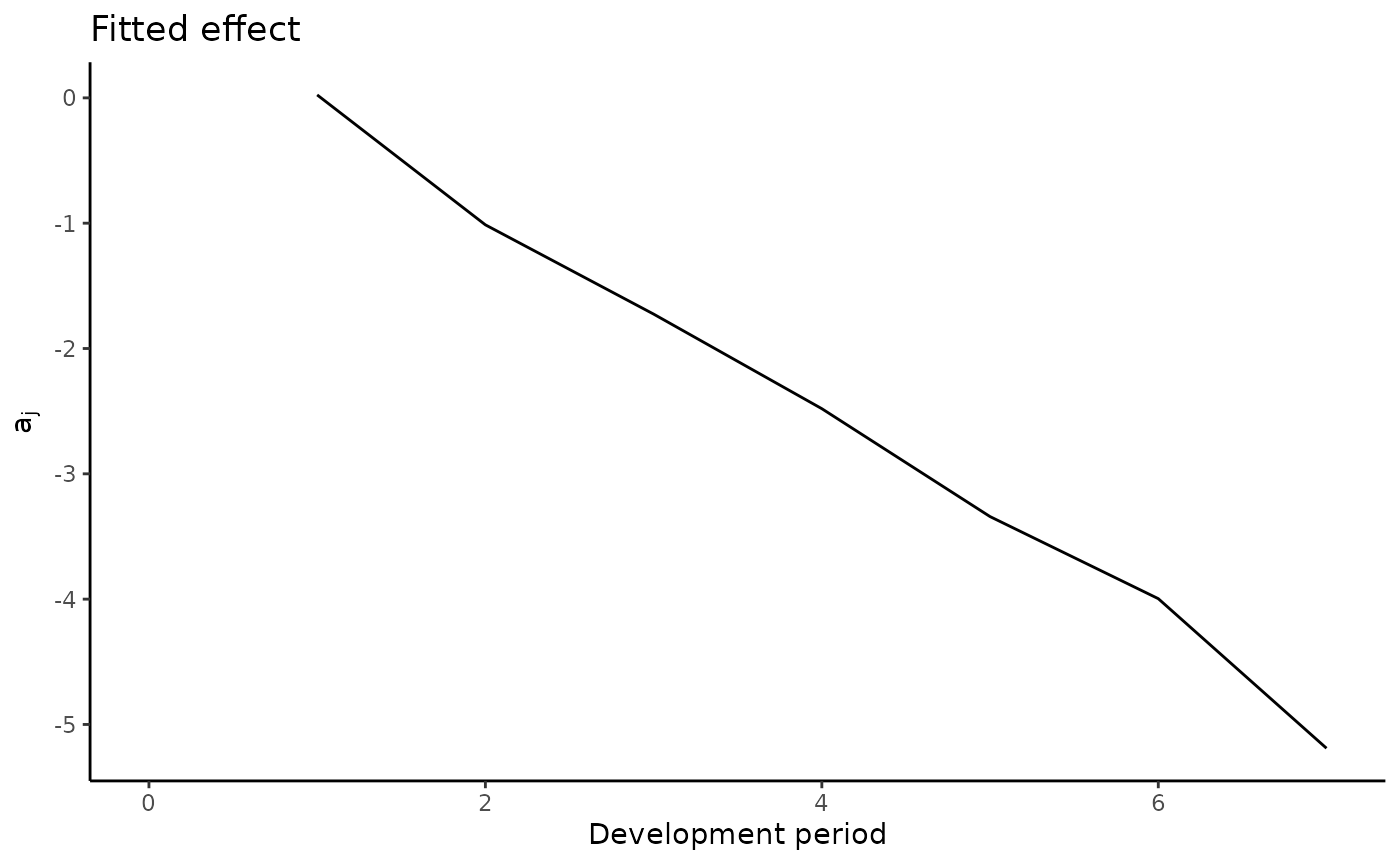

Fitted effect by development period, age-model.

Adding a cohort effect on the claim development model

By adding a cohort component to the claim development model, we improve the scaled-deviance residuals. The scaled-deviance residuals can be plotted using the plot function on the output of the clmplus method.

#make it triangular
plot(a.model.fit)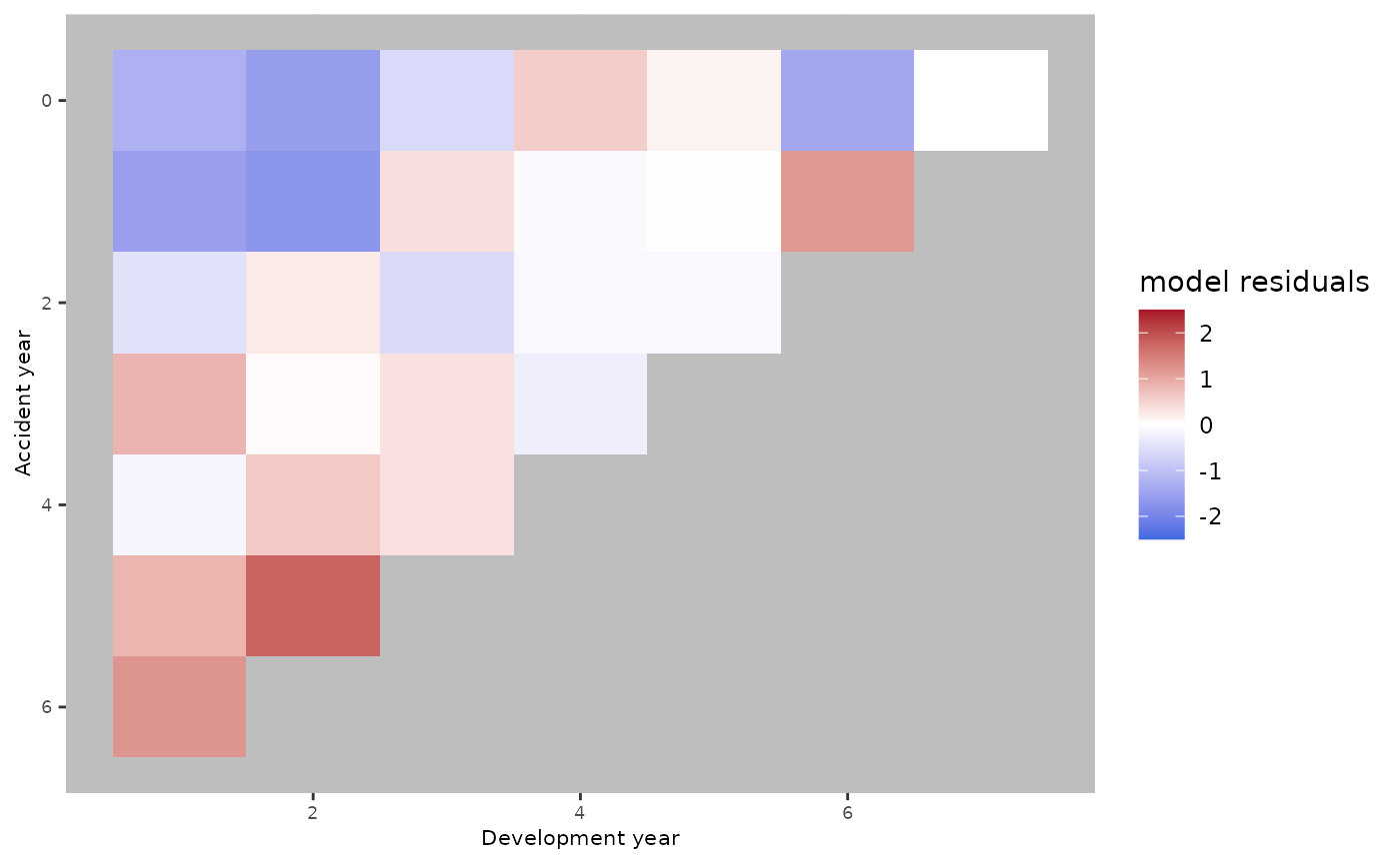

Scaled deviance residuals, age-model.

The red and blue areas suggest that there are some trends that the age-model wasn’t able to catch.

ac.model.fit <- clmplus(pp_data, 
                    hazard.model="ac")
#> StMoMo: The following ages have been zero weighted: 1 
#> StMoMo: The following years have been zero weighted: 1 
#> StMoMo: The following cohorts have been zero weighted: -7 -6 -5 -4 -3 -2 -1 7 
#> StMoMo: Start fitting with gnm
#> StMoMo: Finish fitting with gnm

ac.model <- predict(ac.model.fit,
                    gk.fc.model='a')
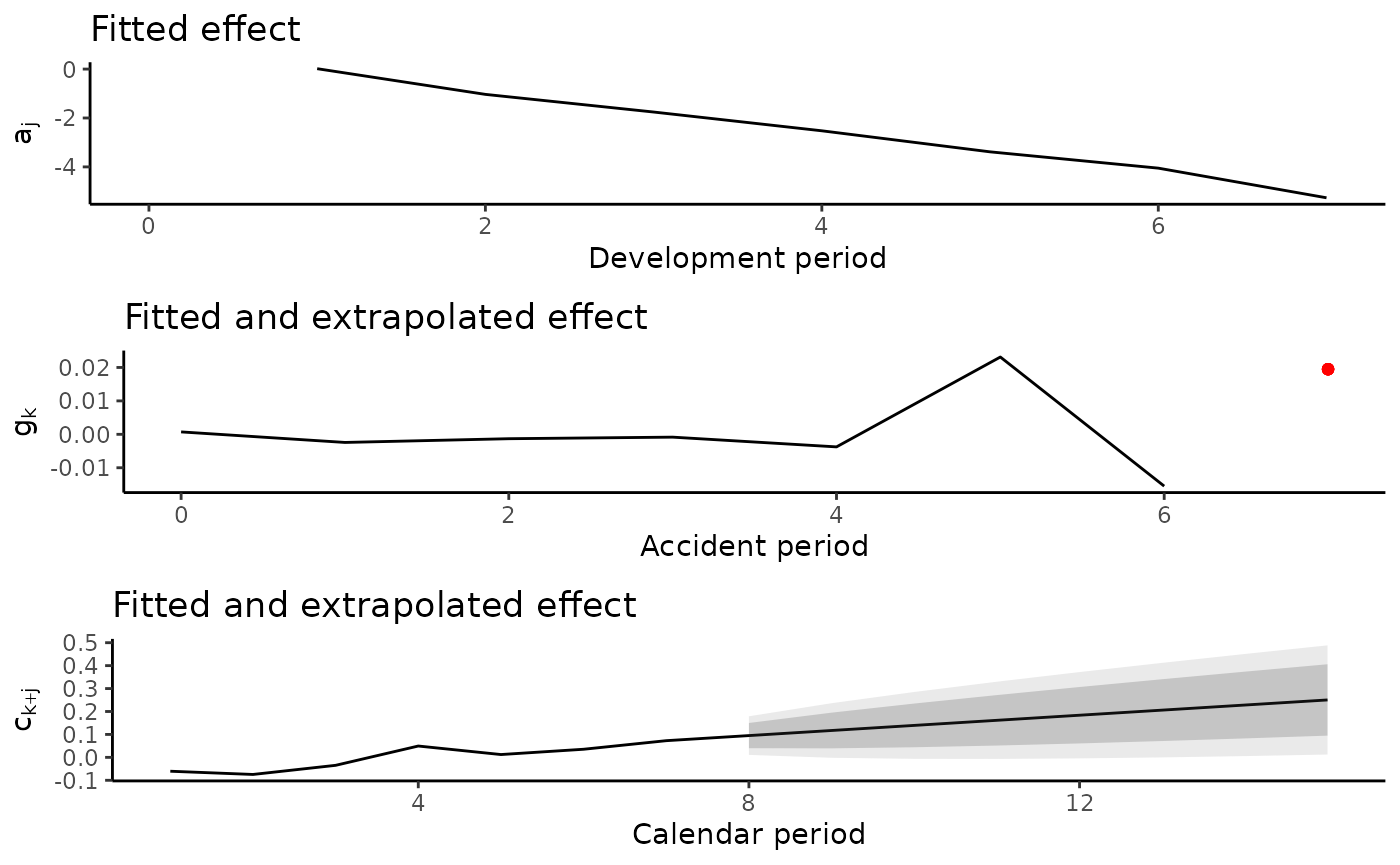
plot(ac.model.fit)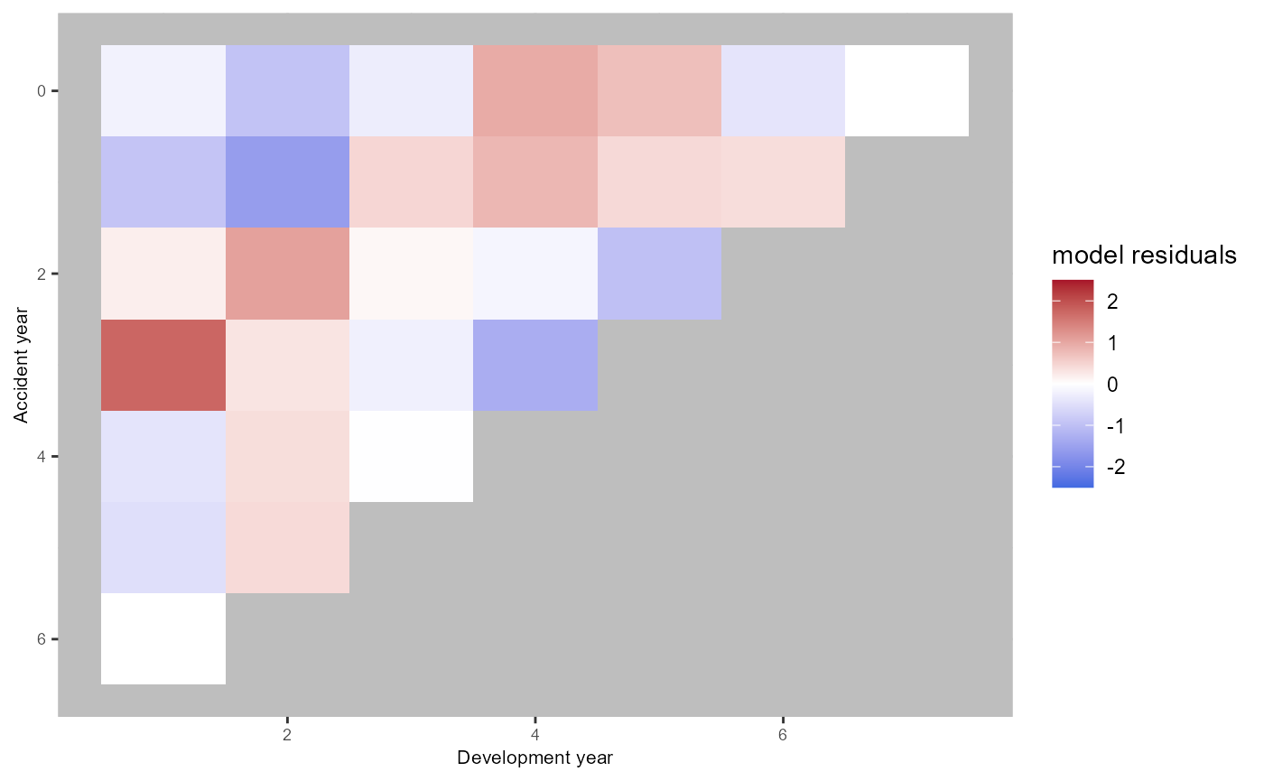

Scaled deviance residuals, age-cohort model. The fitted effect are displayed below. The cohort component is extrapolated for the last available accident period as discussed in our paper.


plot(ac.model)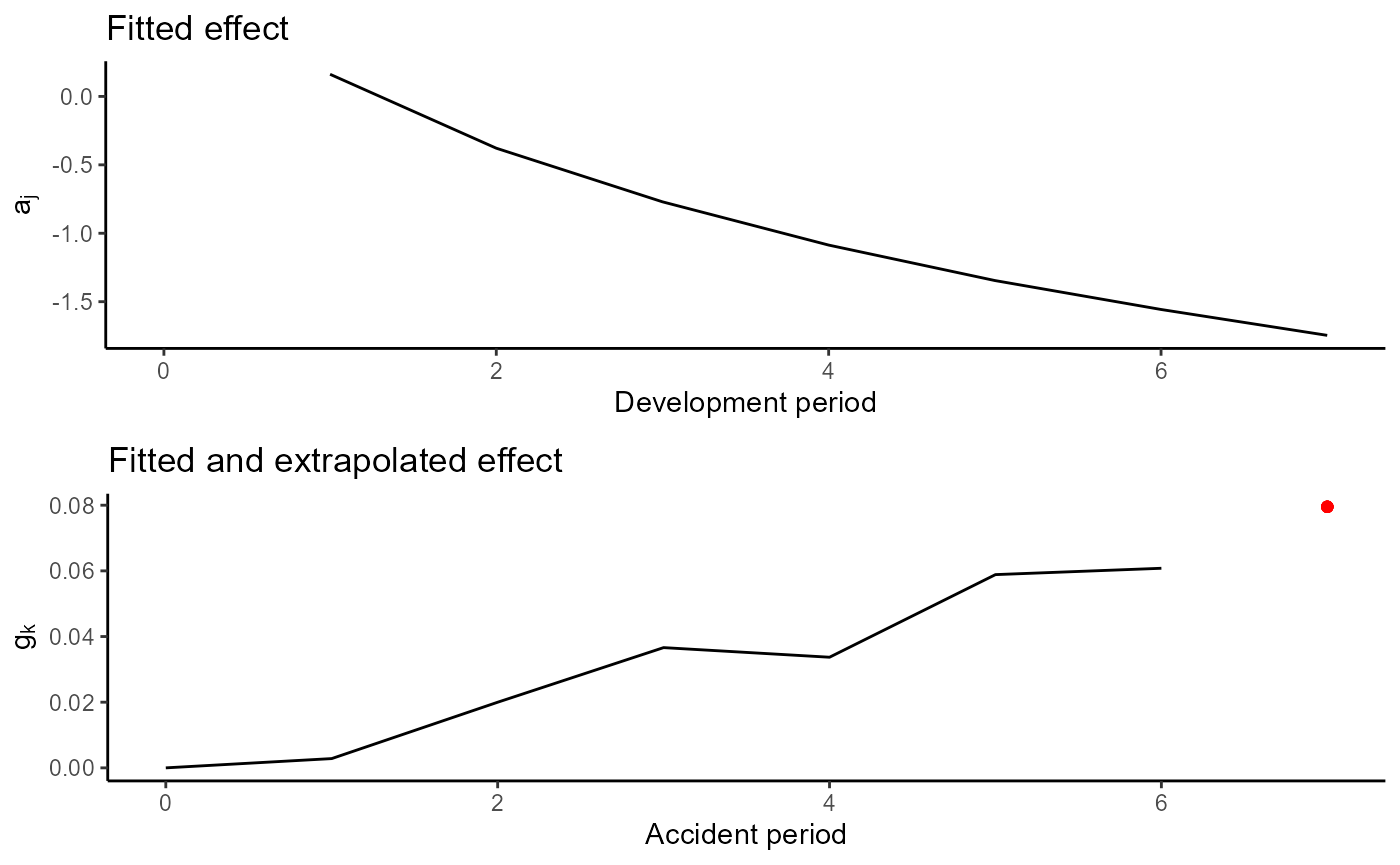

Fitted effects, age-cohort model.

Modelling a period effect on the claim development

It is also possible to add a period component and choose an age-period model or an age-period-cohort model.

ap.model.fit = clmplus(pp_data,
                   hazard.model = "ap")
#> StMoMo: The following ages have been zero weighted: 1 
#> StMoMo: The following years have been zero weighted: 1 
#> StMoMo: The following cohorts have been zero weighted: -7 -6 -5 -4 -3 -2 -1 7 
#> StMoMo: Start fitting with gnm
#> StMoMo: Finish fitting with gnm

ap.model<-predict(ap.model.fit, 
                   ckj.fc.model='a',
                   ckj.order = c(0,1,0))

apc.model.fit = clmplus(pp_data,hazard.model = "apc")
#> StMoMo: The following ages have been zero weighted: 1 
#> StMoMo: The following years have been zero weighted: 1 
#> StMoMo: The following cohorts have been zero weighted: -7 -6 -5 -4 -3 -2 -1 7 
#> StMoMo: Start fitting with gnm
#> StMoMo: Finish fitting with gnm

apc.model<-predict(apc.model.fit, 
                   gk.fc.model='a', 
                   ckj.fc.model='a',
                   gk.order = c(1,1,0),
                   ckj.order = c(0,1,0))

There is no clear difference between the residuals plot obtained using an age-period model compared to the residuals plot obtained using the age-cohort model. Conversely, the plot seems to improve using an age-period-cohort model.

plot(ap.model.fit)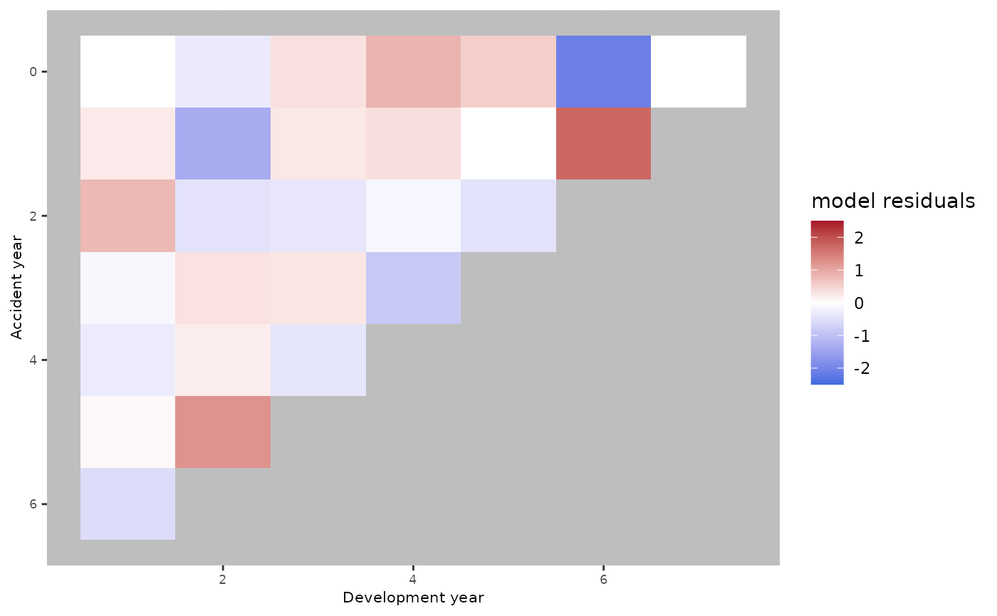

Scaled deviance residuals, age-period model.

plot(apc.model.fit)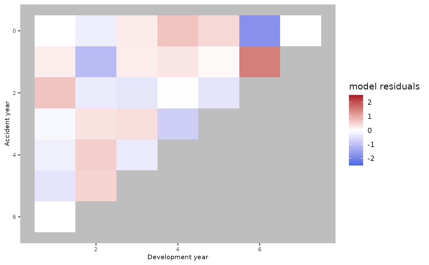

Scaled deviance residuals, age-period-cohort model.

Below, the effects of the age-period-cohort model.

plot(apc.model)

Fitted effects, age-period-cohort model.

References

England, Peter, and Richard Verrall. 1999. “Analytic and Bootstrap Estimates of Prediction Errors in Claims Reserving.” Insurance: Mathematics and Economics 25 (3): 281–93.

Fannon, Zoe, and Bent Nielsen. 2020. Apc: Age-Period-Cohort Analysis. https://CRAN.R-project.org/package=apc.

Gesmann, Markus, Daniel Murphy, Yanwei (Wayne) Zhang, Alessandro Carrato, Mario Wuthrich, Fabio Concina, and Eric Dal Moro. 2025. ChainLadder: Statistical Methods and Models for Claims Reserving in General Insurance. https://CRAN.R-project.org/package=ChainLadder.

Mack, Thomas. 1993. “Distribution-Free Calculation of the Standard Error of Chain Ladder Reserve Estimates.” ASTIN Bulletin: The Journal of the IAA 23 (2): 213–25.

Pittarello, Gabriele, Munir Hiabu, and Andrés M Villegas. 2025. “Replicating and Extending Chain-Ladder via an Age–Period–Cohort Structure on the Claim Development in a Run-Off Triangle.” North American Actuarial Journal, 1–31.

Gabriele Pittarello

2025-06-12

Introduction

Replicate the chain-ladder with the `clmplus` package

Claims reserving with GLMs compared to hazard models

Adding a cohort effect on the claim development model

Modelling a period effect on the claim development

References

Vignette 1

Gabriele Pittarello

2025-06-12

Introduction

Replicate the chain-ladder with the clmplus package

Claims reserving with GLMs compared to hazard models

Adding a cohort effect on the claim development model

Modelling a period effect on the claim development

References

Replicate the chain-ladder with the `clmplus` package